Next: Error sensitivity Up: Tomography Previous: Introduction Contents
Resolution
This section analyses the resolution of the tomographic model system
outlined in the previous section both by singular value
decomposition and model tests.
In paper I, I tried to apply the standard method of calculating the 3-D
resolution for ALIS by singular value decomposition (SVD). Due to the
curse of dimensionality the number of voxels had to be reduced from
![]() to
to ![]() and the number of pixels per image had to be
reduced from
and the number of pixels per image had to be
reduced from ![]() to
to ![]() thus restricting the possible
conclusions about the three-dimensional resolution.
thus restricting the possible
conclusions about the three-dimensional resolution.
Now with the two-dimensional tomographic model system with imaging
stations at 50 km north, 0, 50 and 100 km south, it is possible to
apply the SVD analysis with a vertical slice with 128 voxels per side
and one-dimensional images with 256 pixels. With the
cameras directed towards the centre of the voxel slice, the
transfer matrices from the stations ![]() have been
calculated. Concatenating the station transfer matrices gives a full
system transfer matrix:
have been
calculated. Concatenating the station transfer matrices gives a full
system transfer matrix:
With SVD analysis the resolution in voxel space can
be calculated. Given the transfer matrix
![]() from the voxel space down to all images
with a singular value decomposition
from the voxel space down to all images
with a singular value decomposition
![]() , the
maximum spatial resolution is given by the resolution matrix
, the
maximum spatial resolution is given by the resolution matrix
![]() ( Menke, 1989).
( Menke, 1989).
In order to suppress noise in the reconstruction, only the ![]() singular values
larger than 1 in the singular value decomposition of
singular values
larger than 1 in the singular value decomposition of
![]() above are kept. To illustrate the result of
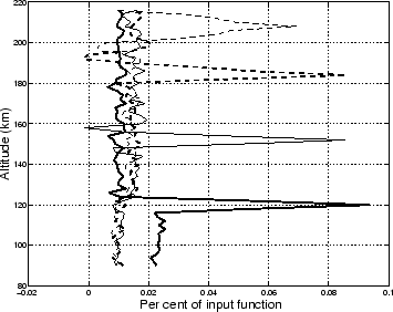
the SVD analysis, we calculate the point spread of three input points
at altitudes of 120, 152 and 184 km central in the slice. By doing this
we get the variation of the point spread function with altitude.
above are kept. To illustrate the result of
the SVD analysis, we calculate the point spread of three input points
at altitudes of 120, 152 and 184 km central in the slice. By doing this
we get the variation of the point spread function with altitude.
 |
Next: Error sensitivity Up: Tomography Previous: Introduction Contents
copyright Björn Gustavsson 2000-10-24

