Next: Resolution Up: Tomography Previous: Tomography Contents
Introduction
One of the main purposes of ALIS is to determine the full 3-D spatial structure of the aurora. This cannot be done with measurements from a single station and this is the main reason for developing ALIS as a multi-station system, with as many stations as possible to optimise the coverage of northern Scandinavia. This system gives simultaneous images of the aurora seen from different perspectives.
This chapter presents a short introduction to three-dimensional tomographic methods. Further it investigates the tomographic resolution of a ground-based system and the error sensitivity of such a system, and describes a general stopping criterion that gives a sufficient condition for when to interrupt iterative solutions for tomography.
![\begin{figure}
\vspace{-.5cm}
\epsfxsize =4.cm
\mbox{\epsffile {Figures/tomo_prob.ps}}
%\caption[The ground-based tomographic problem]{}
\end{figure}](img104.gif) |
where
 |
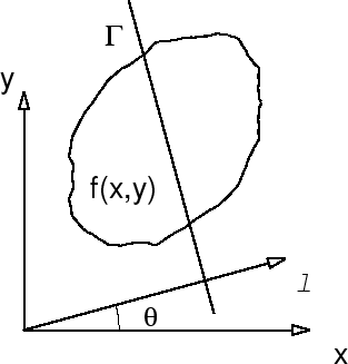
It is possible to obtain an exact and unique solution of the source
function ![]() if and only if
if and only if
![]() is known for all
rays
is known for all
rays ![]() that cut the region where
that cut the region where ![]() . That is for an
angle
. That is for an
angle ![]() we have to move the detector along
we have to move the detector along ![]() so that
measurements are made for all rays that go through the object. The
solution can be written as ( Gordon and Herman, 1974):
so that
measurements are made for all rays that go through the object. The
solution can be written as ( Gordon and Herman, 1974):
For the three-dimensional tomographic problem exact solutions can be
obtained if there is an observation point from which our image
projections are made on every plane
that cuts the region where the function
![]() ( Kudo and Saito, 1990; Smith, 1990). There exist a number of analytical
algorithms that determine
( Kudo and Saito, 1990; Smith, 1990). There exist a number of analytical
algorithms that determine ![]() from a set of image projections which
closely satisfy the above condition ( Jacobsson, 1996; Grangeat, 1990).
from a set of image projections which
closely satisfy the above condition ( Jacobsson, 1996; Grangeat, 1990).
However, in most cases these tomographic problems are ill-posed, meaning that they are sensitive to noise in the measurements or have either an infinite number of exact solutions or no exact solutions. With some regularization schemes, i.e. physical or mathematical constraints, the problem can, in a restricted sense, be transformed into a well-posed problem ( Ghosh Roy, 1991). Auroral and airglow tomography from ground-based multi-station measurements is ill-posed because only a few projections/images of the aurora are available and that the image data are all taken from below the object and thus are close to being linearly dependent.
The tomographic problem of ALIS is three-dimensional, and all performance,
resolution and error analysis on the actual geometry suffers badly from
the curse of dimensionality. That is, the total size of the
tomographic problem is proportional to the total number of pixels in
the images times the total number of volume elements (voxel = volume
element, small cube, c.f. pixel = picture element) in the retrieved
volume distribution. For a two-dimensional tomographic problem with
![]() voxels per side, the number of unknowns is
voxels per side, the number of unknowns is ![]() projected onto
projected onto
![]() images with
images with ![]() pixels per one-dimensional image; the size of
the problem is
pixels per one-dimensional image; the size of
the problem is
![]() . For a three-dimensional tomographic system
the total number of pixels is
. For a three-dimensional tomographic system
the total number of pixels is
![]() and the number of voxels
rises to
and the number of voxels
rises to ![]() , giving a total size of the problem of
, giving a total size of the problem of
![]() . For systems studying the ionosphere the
typical number of stations appears to be approximately 5 and typical
number of pixels is 1000 per image dimension. For the retrieved
volume distribution the number of voxels per side is of the
order of 100. When we go from a two-dimensional to a three-dimensional
tomographic problem the total size of the problem
increases by a factor
. For systems studying the ionosphere the
typical number of stations appears to be approximately 5 and typical
number of pixels is 1000 per image dimension. For the retrieved
volume distribution the number of voxels per side is of the
order of 100. When we go from a two-dimensional to a three-dimensional
tomographic problem the total size of the problem
increases by a factor
![]() .
.
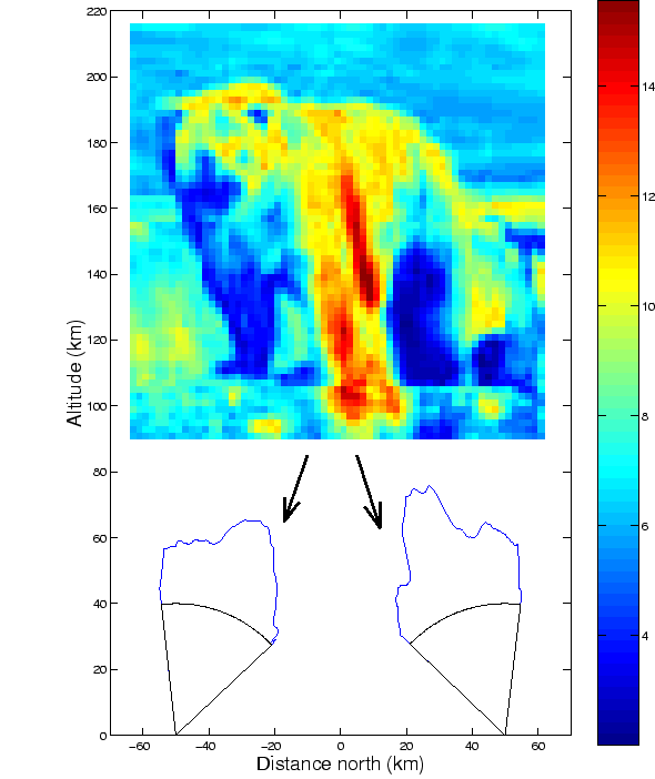
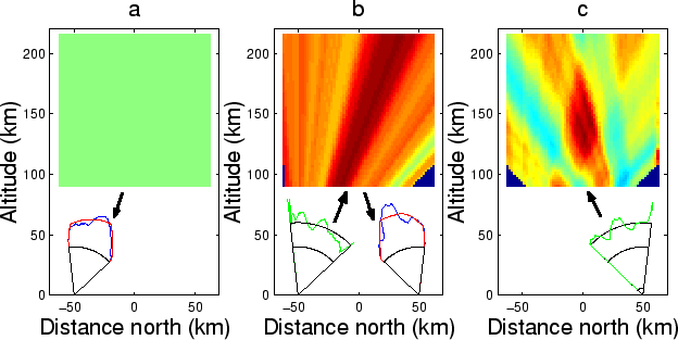
To simplify the analysis in this and the following two chapters, which describe the geometrical calibrations and the forward model, we will study a two-dimensional problem where emission distribution is to be determined in a vertical two-dimensional slice from one-dimensional images. This tomographic model system makes one-dimensional image measurements with the imaging characteristics of the ALIS cameras from four ground-based stations separated by 50 km from each other. The principles of tomographic inversion and all the characteristics of ground-based auroral tomography remain in this 2-D problem but the size is small enough to allow use of the most rigorous analysis of its resolution and retrieval characteristics.
Since ALIS currently only has six ground-based stations, and thus is very far from fulfilling the necessary requirements for obtaining exact reconstructions, we turn to approximate methods in order to obtain the best solution possible.
In order to be able to solve the tomographic problem it is necessary to have good knowledge about the forward problem or forward model. That is, we must know what fraction of the photons emitted in a volume element will be detected and where in the image the intensity will appear. In this model case we have to know how the auroral distribution in a slice is projected down onto the images, as depicted in Figure 3.3.
 |
where
where
If we solve the tomographic problem analytically, we will encouner the problem that the forward model is not a deterministic process, but rather a random process
where a component
where
is the probability that a photon is emitted towards the front lens of camera
Thus we see that the imaging process is a stochastic one for which the
probability of getting a set of measured images ![]() from a
source distribution
from a
source distribution ![]() is:
is:
where
The solution to the inverse problem is then to find the
source distribution
![]() that is most probable given
the measurements
that is most probable given
the measurements
![]() and considering
equation (3.9) and Bayes' rule the resulting problem is
and considering
equation (3.9) and Bayes' rule the resulting problem is
This is the maximum likelihood solution of the inverse problem. For this case in which the random processes have normal distributions the maximum likelihood solution is the well-known least square solution. For the three-dimensional inverse problem the system transfer matrix
The simple and robust iterative methods we have chosen are the
algebraic reconstruction technique (ART) and the simultaneous
iterative reconstruction technique (SIRT) ( Gordon and Herman, 1974). The
working principle of ART is then to take an initial guess
![]() and project that guess down to an image by
and project that guess down to an image by
Then the current solution
This is a modified multiplicative ART update where the update is a weighted average of the ratios of the measured image
 |
ART is a reconstruction scheme that converges fast but is
sensitive to noise in the images ( Aso et al., 1993). A modified version
is SIRT for which the current guess/solution ![]() is projected down
to all stations at once and the voxel intensity in the reconstruction
is updated with the average ratio of pixels from all stations.
is projected down
to all stations at once and the voxel intensity in the reconstruction
is updated with the average ratio of pixels from all stations.
It is possible to use a priori knowledge about the aurora, such as field-alignedness of the auroral structures ( Semeter, 1997; Aso et al., 1990), in the reconstruction process in order to bias the reconstruction and to avoid noise amplification thereby stabilising the solution. Several more general constraints can also be used to reduce the effect of noise in the images, e.g. spatial low pass filtering in 3-D as outlined in paper I, horizontal median filtering, horizontal smoothing of field aligned intensity variation Aso et al. (1993).
Several more advanced iterative schemes exist and the technically interested reader is directed to Veklerov and Llacer (1989b).
Next: Resolution Up: Tomography Previous: Tomography Contents
copyright Björn Gustavsson 2000-10-24


