HF pump-enhanced airglow

By transmitting a powerful high-frequency (HF) (``short-wave'') radio signal into the ionosphere it is possible to modify the ionosphere given that the ionospheric conditions are favourable (i.e. high enough electron concentration, and little or no auroral activity). Such experiments may excite plasma processes on a wide range of temporal and spatial scales [Leyser et al., 2000]. It is possible to produce enhanced optical emissions, which are far to weak to be detected by the unaided human eye, but that can be detected with sensitive imagers and photometers. These optical emissions can be used as a diagnostic tool to study electron energisation during driven plasma turbulence. For example, it is possible to study what the roles of heating and electron acceleration are for dissipating the turbulence [Leyser et al., 2000]. The naturally occurring airglow emissions at 6300 Å and 5577 Å (from the two lowest excited states of oxygen, $O(^1D)$ and $O(^1S)$) can be enhanced by transmitting a high-powered short-wave radio signal into the ionospheric F-region plasma. The low noise and high quantum-efficiency of the ALIS imager (Chapter 3) makes ALIS an ideal instrument for studying optical effects from active ionospheric experiments.

HF pump-enhanced airglow ^6.3 has been studied at low latitudes (Arecibo, Puerto Rico) since the early 1970s by Carlsson et al. [1982] and Bernhardt et al. [1989]. At mid-latitudes, experiments have been carried out in: Platteville, U.S.A., [Sipler and Biondi, 1972; Haslett and Megill, 1974], Moscow, Russia, [Adeishvili et al., 1978], and in Sura, Russia [Bernhardt et al., 1991]. However, at high (auroral) latitudes, there was only one previous report of HF pump-enhanced airglow before 1999 made by Stubbe et al. [1982].

The airglow enhancement has been attributed to excitation of metastable states of atomic oxygen by energetic electrons accelerated in plasma instabilities, [Gurevich et al., 1985; Perkins and Kaw, 1971; Weinstock and Bezzerides, 1974; Weinstock, 1975] and by energetic electrons from the tail of the heated thermal electron plasma [Mantas and Carlson, 1996; Gurevich and Milikh, 1997; Mantas, 1994]. Electron collisions with energies above 3.5 eV yield the excited $O(^1D)$ metastable state, which radiates at 6300 Å [Bernhardt et al., 1991]. The second excited metastable state $O(^1S)$, which radiates at 5577 Å, is obtained for electron energies from about 4.5 eV and upwards. For comparison, the ionospheric background electron temperature is typically 0.1-0.2 eV. Further, it has been proposed that the $O(^1D)$ state may be thermally excited and that the scarcity of observations of simultaneous 6300 Å and 5577 Å enhancements imply that acceleration of electrons may require special experimental and ionospheric conditions that are not often fulfilled [Mantas and Carlson, 1996].

The EISCAT Heating facility

The EISCAT Heating facility is located at Ramfjordmoen near Tromsø, Norway ( $69.6^{\circ}$N, $19.2^{\circ}$E, $86.3$ m above sea level, L=6.2, magnetic dip angle I= $78^{\circ}$) [Rietveld et al., 1993]. The facility is located about 200 km north of Kiruna (See Figure 6.2). Up

Figure 6.2: Geometry of the HF pump-enhanced airglow. Some of the ALIS stations (see text) observed pump-enhanced airglow over the EISCAT Heating facility. Inset: A vertical cut along the Tromsø-Kiruna meridian. The dot indicates the anticipated region of enhanced airglow and the solid lines indicate the field-of-view of the cameras. [After Figure 1 in Brändström et al., 1999]

to 1.2 MW of CW power in the frequency range from 3.85 to 8 MHz can be generated by twelve transmitters of 100 kW each. There are three antenna arrays, covering the frequency ranges of 5.4-8 MHz, 3.85-5.65 MHz and 5.4-8 MHz. Array 1 has a beam width of $7\hbox{$^\circ$}\xspace$ with a gain of 30 dB corresponding to 1200 MW Effective Radiated Power (ERP). Arrays 2-3 have beam widths of 14.5$^\circ$, a gain of 24 dB and a maximum ERP of 300 MW. The main HF wave parameters such as frequency, polarisation, beam direction, and maximum power are chosen and set up at the time of tuning-up the transmitters. It is furthermore possible to modulate, power-step, change polarisation modes and to change the direction of the beam during an experiment [Rietveld et al., 1993].

The EISCAT Heating facility enables strong excitation of plasma turbulence in a wide range of angles to the geomagnetic field. This is due to the fact that the pump electric field is directed parallel to the geomagnetic field at the reflection height, and essentially perpendicular to the magnetic field at only a few kilometres lower altitude [Leyser, 1991].

ALIS observations of enhanced airglow

Starting in 1995, a series of experiments were carried out, attempting to produce enhanced airglow with the EISCAT Heating facility, and to detect it with ALIS. Stubbe et al. [1982] noted that such experiments require: a sufficiently high ionospheric critical frequency, dark and clear skies, no auroral activity and a low or at least stable natural airglow background. As seen from Table 6.4 many events are yet to be analysed. In the following text emphasis will be on the 16 February 1999 event.

Table 6.4: An overview of most HF pump-enhanced airglow experiments carried out with ALIS. The column HEA indicates if HF pump-enhanced airglow was observed. Question marks indicate uncertainty at the time of observation. As seen, the events which have proved most interesting so far are 16 February 1999 and 21 February 1999. Analysis and new measurements are still in progress as this is written.

Observations on 16 February 1999

The first unambiguous observation of HF pump-enhanced airglow at auroral latitudes was made on 16 February 1999 [Brändström et al., 1999]. This evening the skies were clear at most ALIS stations and there was no auroral activity ( $K_p \approx 0$). ALIS operated between 16:15 and 18:30 UTC taking a new image every 10 s with 5 s integration time for the $O(^1D)$ 6300 Å emission line. The sensitivity of the CCD-cameras was enhanced 64 times by on-chip binning $8\times 8$ pixels, thus reducing the spatial resolution from $1024 \times 1024$ pixels to $128 \times 128$ pixels. All ALIS-cameras were pointing towards the anticipated region of enhanced airglow. This is the so called ``heating-position'' (see Table 3.6 and Figure 3.11), centred at an altitude of approximately $250$ km above the EISCAT Heating facility (Figure 6.2). Ten transmitters were operating with an output power of 85 kW each. Thus a total transmitted power of 850 kW, yielded an ERP of around 125 MW. The transmitted frequency was 4.04 MHz, reflecting in the ionospheric F-region, and the ordinary mode (O-mode) beam was tilted $6\hbox{$^\circ$}\xspace$ south from the vertical (which is about half the angle between the vertical and the geomagnetic field in the ionospheric F-region above the transmitters). The transmitters (or ``HF-pump'') were cycled on/off with a duty cycle of 50%. Between 16:32 and 17:22 UTC the transmitters were cycled 2 min on/2 min off. Between 17:24 and 18:32 UTC this was changed to 4 min on/4 min off.

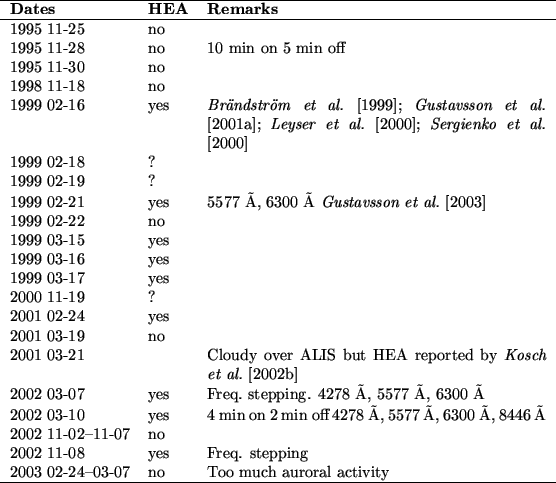When the transmitters were cycled 2 min on/2 min off, weak airglow enhancements were observed [Brändström et al., 1999; Gustavsson et al., 2001a; Leyser et al., 2000]. Starting at 17:32 UTC and continuing until 18:30 UTC (transmitters 4 min on/4 min off) pump-enhanced airglow was observed by all ALIS stations in operation. Due to occasional thin clouds and technical problems, some data-losses occurred. In Figure 6.3 the maximum

Figure 6.3: Maximum and average column emission of the 6300 Å airglow as seen from four stations. The intensity modulations correlate well with the transmitter-on/off cycles. After 17:40 UTC the Kiruna camera was directed to local zenith, imaging the natural background airglow. [After Figure 1 in Gustavsson et al., 2001a]

intensity of the 6300 Å emission is plotted against time for each image from the four stations observing between 16:40 and 18:40 UTC.

The airglow intensity has an $e$-folding growth time of about 60 s after transmitter-on, and decays with an $e$-folding decay time of about 35 s after transmitter-off. After the growth time following transmitter-on, the maximum intensity of the emission appears to have a different temporal evolution at different transmitter-on/off periods. This feature may be due to irregularities in the background ionosphere, which drift through the transmitted beam.

A series of images of the airglow intensity is shown in Figure 6.4.

Figure 6.4: Sequence of airglow images from the Silkkimuotka ALIS station for 20 s intervals following transmitter-on at 17:40:00 UTC (top), and at 10 s intervals following transmitter-off at 17:44:00 UTC (bottom). The intensity scale is in raw counts. Two peaks of airglow intensification are clearly visible in the transmitter-on sequence. [After Figure 3 in Brändström et al., 1999]

Transmitter-on occurs at 17:40 UTC, beyond which the airglow region and intensity is seen to slowly grow, forming two peaks. The upper one appears to saturate, after which the lower peak underneath intensifies, and eventually merges with the first peak. Transmitter-off occurs at 17:44 UTC, beyond which the airglow slowly decays. The peak intensity was estimated to be approximately $300 \pm 100$ R. (See Section 4.2.1, regarding the estimated error of the absolute calibration).

Figure 6.5 shows data from the Silkkimuotka station

Figure 6.5: A series of images of enhanced 6300 Å airglow recorded at the Silkkimuotka station for the period 1748-1752 UTC. The upper panel displays an image sequence just after transmitter-on, and the lower panel shows images near transmitter-off. [After Figure 3 in Leyser et al., 2000]

obtained near transmitter-on at 17:48:00 UTC and -off at 17:52:00 UTC. Both the intensity and size of the patch are seen to slowly increase after transmitter-on, and to decay slowly after transmitter-off.

From Figure 6.3 it is seen that simultaneous data from up to three stations exist for some time periods. This enables triangulation of the height of the airglow region. As shown in the top panel in Figure 6.6, the typical height of the

Figure 6.6: The upper panel shows the triangulated altitude of maximum enhanced airglow. The thick dashed line represents the altitude of the enhanced ion line as observed by EISCAT. The lower panels shows the horizontal location relative to Kiruna of the enhanced airglow region for the corresponding pulse. The dashed contours are the projections of the -1 and -3 dB free space antenna pattern projected to the reflection height. [After Figure 6 in Gustavsson et al., 2001a]

maximum emission was found to be 230-240 km from 17:32 UTC to 18:08 UTC. For the transmitter-on at 18:12 UTC, the enhanced airglow altitude is 250-260 km. In the bottom panel it is shown that the airglow region was positioned approximately 160-170 km to the north of Kiruna and 50 km to the west.

In Figure 6.7, it is seen that the initial location of the

Figure 6.7: Upper left: trajectories of the centres of 6300 Å airglow emission, starting at the black points. Upper right: centres of $O(^1D)$ excitation. Lower left: centres of 6300 Å airglow emission. Lower right: centres of $O(^1D)$ excitation. There are 10 s between the markers in all panels, and all distances are relative to Kiruna. The dashed contours are the -1 and -3 dB projections of the HF-pump beam. [After Figure 4 in Gustavsson et al., 2001a]

two interaction regions are approximately 20-30 km apart. The initially more intensive northernmost region of excitation is fairly immobile, while the southernmost moves 30 km northward in 4 minutes corresponding to a velocity of $100 \pm 20$ m/s [Gustavsson et al., 2001a].

Also, the ionospheric F-region neutral wind was measured by Fabry-Perot interferometers (FPI) [Aruliah et al., 1996; Gustavsson et al., 2001a]. Figure 6.8 displays winds varying

Figure 6.8: Fabry-Perot interferometer measurements of the neutral wind at 240 km altitude. The circle represents the field of view of the FPI looking at $45\hbox{$^\circ$}\xspace$ elevation. This represents a circle above Kiruna with a radius of approximately 240 km. [After Figure 3 in Gustavsson et al., 2001a]

between eastward and north-eastward, with velocities of 130-180 m/s. At 17:45 UTC the wind direction was $42\hbox{$^\circ$}\xspace \pm5\hbox{$^\circ$}\xspace$ (north-eastward) with a velocity of $150\pm5$ m/s. Fabry-Perot neutral wind measurements (Figure 6.8) agree well with the north-eastward drift of the ``centre of emission''.

The EISCAT-UHF radar, operated at about 930 MHz, measured background plasma parameter values. The radar was operating in the common-program-1 mode with a GEN-type long pulse and alternating code [Wannberg, 1993], and was directed parallel to the geomagnetic field [see Leyser et al., 2000, for additional information about the radar measurements].

Figure 6.9 displays these measurements of electron density,

Figure 6.9: EISCAT UHF radar measurements of electron density (top panel), electron temperature (middle panel) and ion temperature (lower panel) on 16 February 1999. The data are for altitude gates spaced 22.5 km apart, which were analysed with 5 s time resolution. The blank areas below 350 km altitude are regions where the ion-line was enhanced by the HF-pump wave, causing the standard analysis to be invalid. [After Plate 3 in Gustavsson et al., 2001a]

electron temperature and ion temperature versus time and altitude, with a range resolution of 22.5 km. Enhanced electron temperature is clearly seen for the transmitter cycle period of eight minutes (17:24-18:32 UTC). The electron temperature rises from an unperturbed background temperature of approximately 1000 K to about 3500 K, which corresponds to an increase of 250%. The exceptionally high temperature measurement at 18:20-18:24 UTC might be contaminated by pump-enhanced ion lines. The temperature enhancement extends several tens of km below the pump reflection height and several hundred kilometres above the reflection height [Leyser et al., 2000]. A decay of the ionospheric electron density is seen in the top panel of Figure 6.9, as expected after sunset.

Discussion

The first report of HF pump-enhanced airglow at high latitudes was made by Stubbe et al. [1982] at the EISCAT Heating facility, Ramfjordmoen, Norway on October 5, 1981 at 17:40-18:20 UTC. In this experiment, photometers recorded a 50% increase (about 20 R ) of the red-line (6300 Å) and a 15% decrease of the green line (5577 Å) during transmitter-on periods. The frequency was 5.423 MHz, and an O-mode beam with an ERP of 260 MW was switched 5 min on/5 min off. However, simultaneous observations made by Henriksen et al. [1984] did not find any evidence of pump enhanced airglow, which casted some doubts on the results by Stubbe et al. [1982]. In both of these observations, the optical instrumentation was scanning photometers with field-of-view of about $5^{\circ}$. This could have introduced aiming problems, causing the photometers to measure in the wrong region of the sky. On the other hand, it must be noted that Radio Frequency Interference (RFI) is more likely to produce false positive results from a photometer, as compared with an imager as a shift of bias of a single readout channel is more likely to be affected than all pixels in an image. These remarks illustrate why multi-station imaging measurements are superior to photometers given enough sensitivity. Such cameras were not available at the time of the experiments cited above.

The first clearly unambiguous observations of high-latitude HF pump-enhanced airglow were made on 16 February 1999, as described in the previous section. The positive result of this and subsequent observations might be attributed to some of the following reasons: improved optical instrumentation, more favourable ionospheric conditions, the approaching solar maximum. While the previous positive observation by Stubbe et al. [1982], relied on photometer measurements made from the same site as the EISCAT Heating facility, the results from 16 February 1999 were obtained by several stations located about 150-200 km away from the heating facility. Therefore, direct RFI from the transmitters can be clearly ruled out for these observations. The observations have also been confirmed by simultaneous measurements from an independent imager [Kosch et al., 2000a; Kosch et al., 2002b; Kosch et al., 2000b] on several occasions. It could therefore be stated that the validity of these observations are beyond all reasonable doubt. In addition, HF pump-enhanced airglow was observed at auroral latitudes at the High Frequency Active Auroral Research Program facility (HAARP) facility in Alaska [Pedersen and Carlson, 2001].

In Brändström et al. [1999] the observations of 16 February 1999 are found to be similar to the observations by Bernhardt et al. [1991] where an 165 MW, 5.828 MHz O-mode beam produced $\ge200$ R of airglow near zenith above the SURA-facility (latitude $56\hbox{$^\circ$}\xspace$N) in Russia.

The two intensity peaks in Figure 6.4, resemble seed irregularities as discussed by Bernhardt et al. [1991]. The drift-pattern of the two intensity peaks (Figure 6.7) is probably associated with electric fields and neutral-wind convection. During the next transmitter-on period 17:48-17:52 UTC, (Figure 6.5) a single patch of enhanced airglow appeared. Leyser et al. [2000] attributes this variability to possible large-scale plasma density irregularities in the pump-plasma interaction region.

The altitude of maximum volume emission is slightly lower than the pump reflection height of approximately 250 km as measured with the Dynasonde and EISCAT-UHF radar. These measurements are consistent with model calculations of the airglow emission altitude for different source altitudes of monoenergetic electrons [Bernhardt et al., 1989].

The observed decay time of the airglow of approximately 30-35 s is significantly shorter than the 110 s lifetime of the $O(^1D)$ metastable state [Solomon et al., 1988]. However, at 240 km altitude, the effective life time of the $O(^1D)$ emission is reduced due to collisional quenching by excitation of vibrational states in $N_2$ and $O_2$ to as low values as 30 s [Sipler and Biondi, 1972; Bernhardt et al., 1991]. Thus, the observed decay time is consistent with the effective life time of the $O(^1D)$ state being reduced by quenching [Leyser et al., 2000].

Sergienko et al. [2000] used EISCAT measurements of the electron temperature to estimate the position and magnitude of the heating source. The magnitude of a modelled electron heating source was adjusted to give the best fit to the observed time-behaviour of the electron temperatures at all altitudes. This procedure led to a determination of the position and magnitude of the electron-heating source at 220 km altitude and $6\times10^4~\mathrm{eV}\mathrm{s}^{-1}~\mathrm{cm}^{-3}$ respectively. A good agreement with the measured and calculated electron temperatures were obtained. The next step was to compare modelled and measured column emission rates of the $O(^1D)$ (6300 Å) line. Assuming a thermal excitation mechanism led to large overestimates of the modelled column emission rates as compared to an accelerated electron excitation mechanism. The paper shows that the assumption of abnormal electron heating generated by the transmitted wave leads to a possible explanation of the observed electron-temperature variations, but cannot account for the observed airglow variations. A process resembling acceleration by Langmuir turbulence (where the electrons above 2 eV are non-Maxwellian with a uniform energy distribution from 3-10 eV) might be an alternative explanation for airglow enhancements. This modelling was done according to the analysis by Bernhardt et al. [1989] and by calculating the production rate of the $O(^1D)$ state by electron impact according to the Monte Carlo model for electron transport into the atmosphere by Ivanov and Sergienko [1992].

It was, however, later found out that the electrons are more likely accelerated by upper hybrid turbulence [see Leyser et al., 2000] instead of Langmuir turbulence. For example, if the pump-frequency is close to a multiple of the electron gyro-frequency, the optical emissions in 6300 Å and 5577 Å becomes very faint [Kosch et al., 2002a] while the Langmuir turbulence is very strong. This is also consistent with results from tomographic inversion, which resulted in a too low altitude for Langmuir-turbulence. [Leyser and Gustavsson, 2003]

The most complete treatment of the observations from 16 February 1999 (so far) is presented in Gustavsson et al. [2001a]. This paper presents the first estimate of the volume distribution the HF pump-enhanced airglow emission obtained from a tomography-like analysis of the image data. Where data from three stations exists (17:40-17:56 UTC), the tomography-like inversion procedure gives reliable results [see Gustavsson et al., 2001a, for details]. For periods with data from only two stations a stereoscopic triangulation method was employed to determine the position of the enhanced airglow region. In Figure 6.10 the result of the tomography-like

Figure 6.10: Volume rendering of the artificially enhanced airglow region above Tromsø, as seen from the west. The bottom plane shows the map of the Tromsø/Kiruna region. The yellow lines are the HF-pump 70% and 10% beam widths in the meriodonal plane, the purple and orange contours are the 6300 Å emission and the $O(^1D)$ excitation. UTC is (from left to right then top to bottom) 17:32:50, 17:33:20, 17:33:50, 17:34:30, 17:34:50, 17:35:20. [After Plate 5 in Gustavsson et al., 2001a]

inversion is presented. The shape of the excitation varies from prolate along the magnetic field to slightly oblate. Also, the existence of two separable regions is clearly seen in the figure. These results were validated by back-projecting images from the reconstructed volume and comparing them to the original images. Comparing the images [see Gustavsson et al., 2001a] gives a typical maximum error of $\pm10$%. Thin drifting clouds in Abisko as well as uncertainties in the relative sensitivities (Chapter 4) of the cameras contribute to the errors.

There are significant differences between the two pulses, as shown by calculating the ``centres of emission and excitation'' (Figure 6.7). The north-eastward drift of the ``centre of emission'' agrees well with the FPI measurements of the neutral wind. These intensity variations and drift patterns indicate that the energy dissipation of the HF-pump wave depends on the background ionosphere.

Calculating the altitude-averaged lifetime according to Bernhardt et al. [1989] an effective lifetime of $25\pm2$ s is obtained during the pulses and $30\pm2$s for the first minute after the pumping. Applying these results, Gustavsson et al. [2001a] made a model-independent estimate of the altitude average excitation distribution according to Bernhardt et al. [1989] displaying a systematic pattern: initially a patchy structure appears, after 15-25 s the excitation grows in a smaller region, where the surrounding region either saturates or decreases, as shown in Figure 6.11.

Figure 6.11: Estimates of the $O(^1D)$ excitation rates for the period just before transmitter-on and the four 10 s periods just after transmitter-on for five pulses. The arrows are the neutral wind direction projected to the images. All images are from the ALIS station in Silkkimuotka. [After Plate 7 in Gustavsson et al., 2001a]

These results show how nicely multi-station spectroscopic imaging of HF pump-enhanced airglow can visualise the complexity and temporal evolution of the pump-ionosphere interaction. Clearly, many more experiments are needed to fully understand the underlying physics.

For periods with image data from only two stations, triangulation with manual identification of corresponding points was employed. This gave an estimate of the maximum emission altitude varying from 230-240 km at 17:32-18:08 UTC, but from the transmitter-on period starting at 18:12 UTC, the height was 250-260 km (Figure 6.6). A reasonable estimate of the error is $\pm 3$ km. Periods with the largest spread in altitude (17:32, 18:04 UTC) occurred when a rise in altitude of the enhanced ion line was observed. The paper also contains a discussion of temporal and intensity variations and a section on theoretical airglow modelling.

From the analysis of the data-set from 16 February, in part summarised above, Gustavsson et al. [2001a] make a plausible claim that the enhanced airglow is not excited by the high-energy tail of a purely Maxwellian electron distribution and raise a number of questions:

• What physical processes control the complex drift pattern?
• What physical process controls the transition from the initial complex excitation structure?
• During what physical conditions can more than one region of strong $O(^1D)$ excitation coexist?

A brief summary of all results obtained hitherto, including some so far unpublished results, is provided in Leyser et al. [2002].

A recent publication [Gustavsson et al., 2003] reports on the first nearly simultaneous observations of HF pump-enhanced airglow at $O(^1D)$ 6300 Å and $O(^1S)$ 5577 Å. These results were obtained during 21 February 1999 at 4.04 MHz, transmitting vertically with an ERP of 73 MW and an 8 minutes transmitter-on/off cycling period. ALIS station 5 in Abisko alternated between 5577 Å and 6300 Å during the same heater pulse. The regions of enhanced airglow are nearly identical, suggesting that the sources of the emissions are co-located in the ionospheric F-region. During the same transmitted pulse an estimated maximum column emission rate of about 40-60 Rayleighs in 6300 Å and with a maximum column emission rate of about 10-20 Rayleighs in 5577 Å were observed. These preliminary results indicate that an intensity-ratio of 5577 Å and 6300 Å of about 0.3-0.4 implies that the excitation is caused by a non-thermal electron population. Previously obtained intensity ratios were 0.05-0.3 [Haslett and Megill, 1974], and 0.08 [Bernhardt et al., 1989].

HF pump-enhanced airglow in the $N^+_{2}$ 1Neg. 4278 Å emission was observed in photometer data from 2001 by Kaila [2003b]. In March 2002 ALIS observed HF pump-enhanced airglow in $N^+_{2}$ 1Neg. 4278 Å. In this experiment the transmitted wave was stepped up and down in frequency through the third harmonic of the ionospheric electron gyro frequency. The airglow was simultaneously imaged with one CCD camera operated at 6300 Å by M. Kosch in Skibotn, and the mobile ALIS station (Section A.8) located at the same place. The ALIS camera recorded emissions in 5577 Å as the frequency was stepped downward through the gyro harmonic, and weaker 4278 Å emissions as the transmitted frequency was stepped up again. This is the first time that pump-enhanced ionisation of the thermosphere has been directly observed. Furthermore, the frequency dependence of the 4278 Å emission gives input to theoretical modelling of electron acceleration for HF-frequencies near the harmonics. It is important in future experiments to be able to reconstruct the volume distribution of the $N^+_{2}$ 1Neg. emission and compare with the volume distribution of for example $O(^1D)$ to study the role of the underlying plasma dynamics perpendicular and parallel to the geomagnetic field [Leyser et al., 2002]. Therefore it is essential to obtain more multi-station measurements with ALIS in the future.