Removing the instrument signature

First it is necessary to remove the instrument signature from the image data. This task is sometime called ``data reduction''. The procedure is to a large extent similar to that followed when reducing astronomical CCD image data [for example Massey, 1992]. In most cases the reduction is carried out first by removing additive effects, and then proceeding with multiplicative effects.

Bias removal

The simplest way to remove the bias is to subtract an image obtained with zero integration time (usually called bias-frame or zero-exposure). However as the bias-frame is subject to the same read noise (Section 3.1.7) as the object-image, this will generally increase the noise by a factor of $\sqrt{2}$. Preparing a bias-correction image by averaging many bias-frames together reduces this problem. As the bias varies over time it would severely impair the temporal resolution if a large number of zero exposures needed to be taken at regular intervals. To remedy this most CCDs are equipped with some extra pixels at the edge of each line. These pixels are shaded from light and thus provide bias information for each line for each image read-out. In the case of the ALIS imager, there are bias-pixels (also called reference pixels, or overscan-strip) for each line of each quadrant on the CCD as indicated in Figure 4.1.

For each pixel, the bias (or DC-level), $\mathit{B}_{ij}$, can be expressed as follows:

$$\mathit{B}_{ij}=\mathit{B}_{Lj}+\mathit{B}_{\overline{Z}ij}+\mathit{B}_{q}+\mathit{B}_{0}\ \left[\mathrm{counts}\right]$$ (4.1)

Here $\mathit{B}_{0}$ is the black-level (or preset bias), as given in Table 4.1. This value is set in the CCD configuration

Table 4.1: Preset bias-levels (black-levels) for the ALIS imagers. The values are obtained from the configuration files for the imagers.

ccdcam	Preset bias $B_{0}$
1	$-25000$
2	$-30758$
3-4	$-30768$
5-6	$-31768$

file (Section 3.3.3).

Bias variations between the four read-out channels can be equalised by subtracting the quadrant bias, $\mathit{B}_{q}$, for each quadrant ( $0 \cdots 3$). This value can be found by averaging pixels from either zero exposure or from the bias-pixels.

$\mathit{B}_{Lj}$ is the overscan-strip correction, which is obtained by selecting good bias-pixels (not all are usable) and averaging them together on each line. The number of bias-pixels varies between the CCDs, as indicated in Table 4.2.

Table 4.2: Total number of pixels and bias-pixels for the six ALIS imagers. The bias-pixels are given per quadrant. The number of imaging pixels is $1024 \times 1024$ for all six CCDs.

ccdcam	Total pixels ( $m \times n$)	Bias-pixels
1-4	$1124\times1024$	$50 \times 512 \times 4$
5	$1056\times1024$	$16 \times 512 \times 4$
6	$1076\times1024$	$26 \times 512 \times 4$

The number of usable bias-pixels varies even more. A suitable smooth function can then be fitted to this averaged bias-column, although this is not done in the current version of the software.

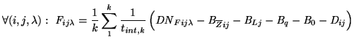
As mentioned initially, to further enhance the bias removal, it is also possible to obtain $k$ bias-frames (Typically at least 25 images), resulting in an averaged bias-correction image, $\mathit{B}_{\overline{Z}ij}$.

$$\forall(i,j) :\ \mathit{B}_{\overline{Z}ij}= \frac{1}{k}\sum_{1}^... ...it{B}_{Lj}-\mathit{B}_{q}-\mathit{B}_{0} \right) \ \left[\mathrm{counts}\right]$$ (4.2)

This correction is normally only present when calibrating the imagers.

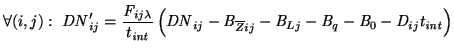
Dark-current

Correction for the dark-current is performed by taking several dark-exposures, i.e. long exposures ( $t_{\mathit{int}}\ge 600$ s) with the shutter closed. The dark-current correction image, $\mathit{D}_{ij}$, is then produced by averaging these images together in much the same way as the averaged bias-correction image (Equation 4.2):

$$\forall(i,j) :\ \mathit{D}_{ij}= \frac{1}{k}\sum_{1}^{k}\frac{1}{... ...thit{B}_{Lj}-\mathit{B}_{q}-\mathit{B}_{0}\right)\ \left[\mathrm{counts}\right]$$ (4.3)

Here $t_{int,k}$ is the integration time for image $k$.

However for the ALIS imagers, this correction has been found to be negligible for integration times less than 10-15 minutes. Therefore, no dark-current correction is made except for very special cases.

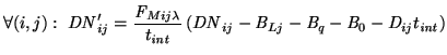
Flat-field correction

The purpose of the flat-field calibration is to remove multiplicative variations introduced by pixel-to-pixel sensitivity differences, vignetting in the optics, variation in transmittance on the filter surface, etc.. This is done by taking a large number of images of a uniform flat-field source:

$$\forall(i,j,\lambda) :\ \mathit{F}_{ij\lambda}= \frac{1}{k}\sum_{... ...ne{Z}ij}-\mathit{B}_{Lj}-\mathit{B}_{q}-\mathit{B}_{0}- \mathit{D}_{ij} \right)$$ (4.4)

In this equation $\mathit{F}_{ij\lambda}$ is the flat-field correction. The index, $\lambda$, indicates that the flat-field correction images should be obtained for each wavelength of interest. Normally this means one set of flat-field images per filter. However a calibration facility which can take measurements for several wavelengths within the filter passband would enable measurements of the combined effects of transmittances (Section 3.1.3) and quantum efficiency (Section 3.1.6) for the entire imaging system (and as a function of wavelength).

The moderate fields-of-view ( $50^{\circ}$- $60^{\circ}$) for the ALIS imagers necessitate an integrating sphere of a sufficient diameter for flat-field calibration [i.e. about 1.5-2 m, see Labsphere, 1997; Brändström, 2000, and references therein.].

Numerous attempts were made to use simpler methods, such as cloudy skies, white screens, diffuse spherical lamp covers etc. to obtain reasonably good flat-field images. None of these attempts provided flat-field images of sufficient quality, as non-uniformities and gradients were hard to avoid with these simple approaches.

One ALIS imager (ccdcam6) has actually been calibrated in the integrating sphere facility at National Institute of Polar Research, Japan [Okano et al., 1997]. The results from this calibration (using white light) are described by Urashima et al. [1999]. Due to the considerable distance to this facility it would be difficult to perform flat-field calibrations for all cameras, as would be required. Therefore it is hoped that a similar calibration facility will be established in the proximity of the optical instruments in northern Scandinavia. This was proposed by Steen [1998]. Such a facility would be beneficial to many imaging devices in Europe.

So far no proper flat-field calibration are done on the ALIS images on a regular basis. Instead, the flat-field correction is solely based on a mathematical model of the vignetting in the optical system [Gustavsson, 2000, Chapter 5]. (This model resembles the ``natural vignetting'' of $\cos^4 \theta$ discussed in Section 3.1.3). Despite the fact that this model does not take variations in filter-transmission, pixel-to-pixel sensitivity variations, etc. into account, it has proved to work reasonably well.

Bad-pixel correction

Defects are unavoidable in the production of a CCD, so defect-free chips are extremely rare and expensive. The CCDs used for the ALIS imagers are of scientific grade, allowing for only a few pixel-defects. The pixel-defects, and how to detect them, can be summarised as follows [after Holst, 1998]:

Point defect:

Pixel with deviation of more than 6 % compared to adjacent pixels when illuminated to 70 % saturation. (Expose a white area to about 70 % of the dynamic range.)

Hot point defect:

Pixels with extremely high output voltage. Typically a pixel whose dark-current is 10 times higher than the average dark-current. (Take a zero or dark image.)

Dead pixels:

Pixels with low output voltage and/or poor responsitivity. Typically a pixel whose output is one half of the others when the background nearly fills the wells. (Expose a white area.)

Pixel traps:

A trap interferes with the charge transfer process and results in either a partial or whole bad line, either all white or all dark. (Take a zero, dark or object image, depending on type of trap)

Column defect:

Many (typically 10 or more) point defects in a single column. May be caused by pixel traps (see above).

Cluster defect:

A cluster (grouping) of pixels with point defects (see above).

Although the CCDs in the ALIS imager are of scientific grade, there are a few pixel-defects present on each CCD. These defects have been identified by manually inspecting the images. The bad pixels are then removed by substituting interpolated values from adjacent pixels.

Summary

The corrections discussed above (apart from the bad-pixel interpolation) are summarised in the following equation:

$$\forall(i,j) :\ \mathit{DN}_{ij}'= \frac{\mathit{F}_{ij\lambda}}{... ...t{B}_{Lj}-\mathit{B}_{q}-\mathit{B}_{0}- \mathit{D}_{ij}t_{\mathit{int}}\right)$$ (4.5)

Here, $\mathit{DN}_{ij}'$ is the corrected pixel value, which is normalised with respect to integration time $t_{\mathit{int}}$.

For most measurements, the following, simplified correction is applied

$$\forall(i,j) :\ \mathit{DN}_{ij}'= \frac{\mathit{F}_{Mij\lambda}}... ...t{B}_{Lj}-\mathit{B}_{q}-\mathit{B}_{0}- \mathit{D}_{ij}t_{\mathit{int}}\right)$$ (4.6)

The symbol, $\mathit{F}_{Mij\lambda}$ is the modelled flat-field correction, as discussed in Section 4.1.3.

Apart from the steps described above, occasionally some additional steps are carried out in order to prepare the data for subsequent analysis. These include various types of filtering to remove cosmic-ray events, stars, etc.