Some basic concepts

There exist a number of textbooks [for example Theuwissen, 1995; Holst, 1998, and references therein], reports [for example Lance and Eather, 1993; Eather, 1982], and articles [for example Janesick et al., 1987, and references therein] on solid-state imaging with CCD detectors. This section will provide a short summary of some fundamental concepts required to specify a CCD-imaging system suitable for the needs of auroral and airglow imaging.

Holst [1998] defines the term radiometry, as the ``energy or power transfer from a source to a detector'' while photometry is defined as ``the transfer from a source to a detector where the units of radiation have been normalised to the spectral sensitivity of the eye.''

Spectral radiant sterance (radiance)

The basic quantity from which all other radiometric quantities can be derived is spectral radiant sterance, $L$. Given a source area, $A_{s}$, radiating a radiant flux, $\Phi$, into a solid angle, $\Omega$. The spectral radiant sterance in energy units, $L_{E}$, then becomes:

$$L_{E}(\lambda)=\frac{\partial^{2}\Phi(\lambda)}{\partial A_{s}\partial\Omega}\ \left[\frac{\mathrm{W}}{\mathrm{m^2\ sr}}\right]$$ (3.1)

where $\lambda$ is the wavelength. Expressing the spectral radiant sterance in quantum units ( $L_{\gamma}$) the following equation is obtained:

$$L_{\gamma}=\frac{L_{E}}{h\nu}=\frac{L_{E}\lambda}{hc}\ \left[\frac{\mathrm{photons}}{\mathrm{s\ m^2\ sr}}\right]$$ (3.2)

Here $\nu$ is the frequency, $h$ is Planck's constant and $c$ is the speed of light. Please note spectral radiant sterance (radiance) is not to be confused with surface brightness which is a photometric unit involving the characteristics of the human eye [see Holst, 1998, pp. 20,26].

The Rayleigh

In terms of measurement techniques the aurora can be regarded as a five-dimensional signal with three spatial dimensions, one temporal and one spectral dimension. The desired physical quantity is usually the volume emission rate, $\epsilon(\mathbf{r},t,\lambda)$, which cannot be found directly from measurements. However the rate of emission from a $1~\mathrm{m}^{2}$ column along the line of sight is normally just $4\pi{}L_{\gamma}$ for any isotropic source with no self-absorption [Hunten et al., 1956].

Consider a cylindrical column of cross-sectional area 1  $\mathrm{m}^{2}$ extending away from the detector into the source. The volume emission rate from a volume element of length $dl$ at distance $l$ is $\epsilon(l,t,\lambda)\ \mathrm{photons}\ \mathrm{m}^{-3}\, \mathrm{s}^{-1}$. The contribution to $L_{\gamma}$ is given by:

$$dL_{\gamma}=\frac{\epsilon(l,t,\lambda)}{4\pi}\,dl\ \left[\frac{\mathrm{photons}}{\mathrm{s\ m^2\ sr}}\right]$$ (3.3)

Integrating along the line of sight, $l$:

$$4\pi L_{\gamma}=\int_{0}^{\infty} \epsilon(l,t,\lambda)dl$$ (3.4)

This quantity is the column emission rate, which Hunten et al. [1956] proposed as a radiometric unit for the aurora and airglow. (See also Chamberlain [1995, App. <]2058#> II#) The unit is named after the fourth Lord Rayleigh, R. J. Strutt, 1875-1947, who made the first measurements of night airglow [Rayleigh, 1930]. (Not to be confused with his father, J. W. Strutt, 1842-1919 remembered for Rayleigh-scattering etc.) In SI-units the Rayleigh becomes [Baker and Romick, 1976]:

$$1\ \mathrm{[Rayleigh]} \equiv 1\ \mathrm{[R]} \triangleq 10^{10} \left[\frac{\mathrm{photons}}{\mathrm{s\ m^2\ column}}\right]$$ (3.5)

The word column denotes the concept of an emission-rate from a column of unspecified length, as discussed above. It should be noted that the Rayleigh is an apparent emission rate, not taking absorption or scattering into account. However, Hunten et al. [1956] emphasise that ``the Rayleigh can be used as defined without any commitment as to its physical interpretation, even though it has been chosen to make interpretation convenient.'' The spectral radiant sterance ( $L_{\gamma}$) in Equation 3.2 can be obtained from the column emission rate $I$ (in Rayleighs) according to Baker and Romick [1976]:

$$L_{\gamma}=\frac{10^{10}I}{4\pi} \left[\frac{\mathrm{photons}}{\mathrm{s\ m^2\ sr}}\right]$$ (3.6)

Although not a proper SI-unit, the Rayleigh is often used in the field of auroral and airglow measurements. It is also frequently misunderstood and abused. It is important to remember that the Rayleigh only is usable when the wavelength is specified. Due to the plethora of Rayleigh definitions [Baker and Romick, 1976], it is always wise to state the definition of the unit before using it. In the following text, the Rayleigh will be used according to the original definition [Hunten et al., 1956, but in SI-units] as defined above.

Using the recommended column emission rates in Rayleighs for the International Brightness Coefficients ( IBC) as an example, the following spectral radiant sterances are obtained [Chamberlain, 1995, App. II]: IBC-I aurora, corresponding to 1 kR at 5577 Å is often described as the lowest column emission rate detectable by the unaided human eye. Usually this is compared to the luminous incidence of a moonless cloudy night which is about $10^{-4}$ Lux^3.1. By the use of Equations 3.2 and 3.6, the spectral radiant sterance in energy units ($L_{E}$) can be calculated:

$$L_{E}(1\ \mathrm{[kR]})=\frac{10^{13} hc}{4\pi\lambda}= \frac{10^{3}hc}{4\pi\times5577} \approx 300 \left[\frac{nW}{\mathrm{s\ m^2\ sr}}\right]$$ (3.7)

Similarly the brightest IBC-IV corresponding to 1 MR at 5577 Å, which is often compared to the luminous incidence of the full-moon of about $10^{-1}$ Lux^3.1 becomes:

$$L_{E}(1\ \mathrm{[MR]})\approx 300 \left[\frac{\mu W}{\mathrm{s\ m^2\ sr}}\right]$$ (3.8)

Spectral radiant incidence (irradiance)

Spectral radiant incidence (irradiance), $E$, is defined as radiant power incident per unit area onto a target, in this case typically the effective aperture of the optics, $A_{app}$, image area, $A_{i}$, area of CCD-detector, $A_{CCD}$, or the area of a CCD pixel, $A_{pix}$.

The transmittance, $T(\lambda,...)$, of an optical system is a function of many parameters, for example wavelength $\lambda$, viewing angle, temperature, etc., and must be experimentally determined (See Chapter 4). Here it is enough to state that the total transmittance is given by the product of the individual transmittances of the various components of the optical system:

$$T=\prod_{\forall X} T_{X}= T_{a} T_{o} T_{f} \ldots$$ (3.9)

Where $T_{X}$ is exemplified by $T_{a}$, $T_{o}$ and $T_{f}$ which are the transmittance of the atmosphere, optics and filter, respectively. In the following text $T$ will denote the product of appropriate transmittances according to Equation 3.9.

Consider an extended source of area, $A_{s}$, of given column emission rate, $I$, imaged by an optical system, here represented by a single lens with given focal length, $f$, and f-number, $f_{\char93 }$. The relation between the aperture-stop, $d_{app}$, f and $f_{\char93 }$ is given by:

$$f_{\char93 }=\frac{f}{d_{app}}$$ (3.10)

Setting the source at distance $r_{s}$ from the lens, which is at the distance $r_{i}$ from the detector and letting $\Omega_{ds}$ be the solid angle of the lens aperture as seen from the source, (assuming small angles), the photon flux, $\Phi_{\gamma_{app}}$, at the lens aperture then becomes:

$$\Phi_{\gamma_{app}}=L_{\gamma}A_{s}T_{a}\Omega_{ds}= L_{\gamma}A_... ..._{a}\frac{A_{app}}{r_{s}^{2}}\ \left[\frac{\mathrm{photons}}{\mathrm{s}}\right]$$ (3.11)

The spectral radiant incidence at the aperture, $E_{\gamma_{app}}$, then becomes:

$$E_{\gamma_{app}}=\frac{\Phi_{\gamma_{app}}}{A_{app}}= \frac{L_{\g... ...A_{s}T_{a}}{r_{s}^{2}}\ \left[\frac{\mathrm{photons}}{\mathrm{s}\ m^{2}}\right]$$ (3.12)

The spectral radiant incidence at the image plane, $E_{\gamma_{i}}$, is given by (by substituting Equation 3.10 and assuming a circular aperture):

$$E_{\gamma_{i}}=\frac{\Phi_{\gamma_{app}}}{A_{i}}= L_{\gamma}\frac... ...{s}^2f_{\char93 }^{2}}\ \left[\frac{\mathrm{photons}}{\mathrm{s}\ m^{2}}\right]$$ (3.13)

Noting that, for thin lenses and small angles:

$$\frac{1}{r_{s}}+\frac{1}{r_{i}}=\frac{1}{f}$$ (3.14)

In this case:

$$r_{s} \gg r_{i} \Rightarrow r_{i} \approx f$$ (3.15)

The lens-magnification formula is:

$$M^{2}=\left(\frac{h_{i}}{h_{s}}\right)^{2}=\frac{A_{i}}{A_{s}}= \left(\frac{r_{i}}{r_{s}}\right)^{2}$$ (3.16)

where $h_{i}$ and $h_{s}$ denote the height of the image and source respectively. Inserting Equations 3.6 and 3.14-3.16 into Equation 3.13, the following equation for $E_{\gamma_{i}}$ is obtained:

$$E_{\gamma_{i}}=\frac{T\Phi_{\gamma}}{A_{i}}= TL_{\gamma}\frac{\pi... ...0}I}{16f_{\char93 }^{2}}\ \left[\frac{\mathrm{photons}}{\mathrm{s\ m^2}}\right]$$ (3.17)

Note that this equation is only accurate for small angles, an off-axis image will have reduced incidence compared to an on-axis image. This is called the ``natural vignetting'', $\cos^4 \theta$, and is usually inserted as a multiplication factor in Equation 3.17, as required.

However, the actual vignetting is highly dependent on the characteristics of the optical system. Therefore the vignetting as well as other aberrations, and the transmittance ($T$) must be experimentally determined. This will be considered further in Chapter 4 and references therein.

Number of incident photons

Using Equation 3.17 the number of photons reaching the image plane, $n_{\gamma_{i}}$, can be calculated:

$$n_{\gamma_{i}}= E_{\gamma_{i}}t_{\mathit{int}}A_{i}= T t_{\mathit{int}}A_{i}\frac{10^{10}I}{16f_{\char93 }^{2}}\ \left[\mathrm{photons}\right]$$ (3.18)

Here $t_{\mathit{int}}$ is the integration time in seconds. The number of photons hitting the CCD, $n_{\gamma_{CCD}}$, are:

$$n_{\gamma_{CCD}}= n_{\gamma_{i}} T_{w} T_{CCD} \frac{A_{CCD}}{A_{i}}\ \left[\mathrm{photons}\right]$$ (3.19)

Here $T_{w}$ is the transmittance of the optical window protecting the CCD, and $T_{CCD}$ is the transmittance of the CCD substrate (in the case of a back-side illuminated CCD). Likewise, the number of photons hitting an individual pixel, $n_{\gamma_{pix}}$, is:

$$n_{\gamma_{pix}}= n_{\gamma_{CCD}}\frac{A_{pix}}{A_{CCD}}= T t_{\... ...{int}}A_{pix}\frac{10^{10}I}{16f_{\char93 }^{2}}\ \left[\mathrm{photons}\right]$$ (3.20)

(using Equations 3.18-3.19 and Equation 3.20). Again, please remember the caution at the end of Section 3.1.3

The CCD as a scientific imaging detector

``During the past couple of decades the Charge Coupled Device (CCD) sensor has gradually replaced the tube type sensors, such as the vidicon, due to its advantages in size, weight, power consumption, noise characteristics, linearity, dynamic range, photometric accuracy, spectral responsitivity, geometric stability, reliability, and durability'' [Janesick et al., 1987]. As an auroral imager, the CCD is thus almost an ideal detector for ground-based as well as for space-borne instruments. The CCD can be used either as the primary photon detector, or in an Intensified CCD (ICCD) configuration. Whether to use a CCD or an ICCD is mainly a matter of requirements on temporal resolution and signal-to-noise ratio, $\mathit{SNR}$. This section will begin with a short review of a number of parameters describing the performance of a CCD detector.

Quantum efficiency

The quantum efficiency, ${Q_{E}}$, is a measure of the number of electrons generated per incident photon:

$${Q_{E}}=\eta_{E}Q_{EI} \left[\frac{e^{-}}{\mathrm{photons}}\right]$$ (3.21)

where $\eta_{E}$ is the effective quantum yield (electrons generated, collected, and transferred per interacting photon per pixel) and $Q_{EI}$ is the interacting quantum efficiency (interacting photons per incident photons per pixel) [Janesick et al., 1987]. However, for the purpose of this text it is only needed to consider ${Q_{E}}$, which for the purpose of this text, is the same as the detective quantum efficiency (DQE).

Quantum efficiency for a CCD is wavelength dependent, and is of no value unless the wavelength is specified. High performance scientific thinned, back-side illuminated anti-reflection coated CCD devices might have as high quantum efficiency as 80-90% in the visible region as demonstrated in Figure 3.1.

Figure 3.1: Quantum efficiency vs. wavelength for the SI-003AB CCD (ALIS ccdcam5) as published in the manufacturers data-sheet. Four curves are presented: with standard anti-reflection coating (``StdAR'') UV anti-reflection coating (``UVAR''), uncoated, thinned, back-side illuminated (``Thinned uncoated'') and front-side illuminated (``Frontside''). The ALIS imagers have a standard anti-reflection coating.

As a comparison, ${Q_{E}}$ for typical consumer CCDs lies in the range 30-70%. The average number of photoelectrons, $\overline{n}_{e^{-}_{\gamma}}$, obtained from $n_{\gamma_{pix}}$ (Equation 3.20) is:

$$\overline{n}_{e^{-}_{\gamma}}={Q_{E}}n_{\gamma_{pix}} \left[e^{-}\right]$$ (3.22)

Noise

Aurora and airglow are so-called photon-limited signals, where the quantum nature of light limits the achievable signal-to-noise ratio. Photon arrival follows Poisson statistics, where the variance is equal to the mean. The sum of the standard deviation of the noise resulting from the photoelectrons, $\langle n_{e^{-}_{\gamma}} \rangle$, and dark-current noise, $\langle n_{e^{-}_{d}} \rangle$, is denoted shot noise, $\langle n_{e^{-}_{s}} \rangle$, and is obtained from the following equation:

$$\langle n_{e^{-}_{s}} \rangle = \sqrt{\mathit{CTE}^{N} \left( \la... ...}\right)} \approx \sqrt{\overline{n}_{e^{-}_{\gamma}}+\overline{n}_{e^{-}_{d}}}$$ (3.23)

Here $\langle {X} \rangle^{2}$ stands for the variance of quantity $X$ and $\langle X \rangle$ is the standard deviation. $\overline{X}$ denotes the mean value. $\mathit{CTE}^{N}$ stands for the Charge Transfer Efficiency ( $\mathit{CTE}$) where $N$ is the number of transfers. Usually $\mathit{CTE}^{N} \approx 1$ for reasonably sized CCD devices. Note that $n_{e^{-}_{\gamma}}$ would be present even for an ideal detector.

Additional noise sources include: reset noise, on-chip and off-chip amplifier noise (1/f-noise and white noise). Of particular interest for low-light applications is that the 1/f-noise, which is the main source of the read noise (``noise-floor''), increases in proportion to the square root of the read-out frequency (``pixel-clock''), thus requiring a suitable compromise between noise performance and frame-rate. The analogue-to-digital converter has a quantisation noise, also switching transients coupled through the clock signals, electro-magnetic interference, etc., sums up to the total noise. There is pattern noise due to differences in dark-current and photo response non-uniformities [Holst, 1998]. At high signal levels the total noise is dominated by pattern noise (pixel to pixel sensitivity variations within the CCD) for most CCDs, at low signal levels the read noise (``noise floor'') dominates [Janesick et al., 1987]. Many of these noise sources can be reduced to negligible levels by good electronic design practices. In particular, the dark-current (and reset noise) is reduced by cooling the CCD. By the use of Double Correlated Sampling (DCS) the reset noise can be almost eliminated. The quantisation noise is eliminated by using a sufficiently high resolution ADC. It is, however, beyond the scope of this work to embark onto a detailed analysis of the noise-sources in CCD imagers, instead a simplified noise model from Holst [1998] is adopted:

$$\langle n_{e^{-}_{CCD}} \rangle =\sqrt{ \langle {n_{e^{-}_{s}}} \... ...}} \rangle^{2}+\langle {n_{e^{-}_{p}}} \rangle^{2}}\ \left[{e^{-}_{RMS}}\right]$$ (3.24)

The standard deviation of the noise floor (or read noise), $\langle n_{e^{-}_{r}} \rangle$, is usually stated in the imager specification as `read noise', or easily obtained from a zero exposure. This noise source increases with the square-root of the pixel clock frequency, which imposes an $\mathit{SNR}$ constraint onto the frame-rate.

The pattern noise, $\langle n_{e^{-}_{p}} \rangle$, is the sum of Fixed Pattern Noise (FPN), resulting from pixel-to-pixel variations in the dark-current, and Photo Response Non-Uniformities (PRNU). An approximate worst case value is provided by Holst [1998]:

$$\langle n_{e^{-}_{p}} \rangle =\sqrt{\langle {n_{e^{-}_{FPN}}} \r... ...line{n}_{e^{-}_{\gamma}}}{\sqrt{{n_{e^{-}_{max}}}}}\ \left[{e^{-}_{RMS}}\right]$$ (3.25)

However, for the low signal levels considered here, pattern noise is neglected. Then the total noise approximation for a bare CCD becomes (by substituting Equation 3.23 into Equation 3.24):

$$\langle n_{e^{-}_{CCD}} \rangle \approx \sqrt{\overline{n}_{e^{-}... ...n}_{e^{-}_{d}}+\langle {n_{e^{-}_{r}}} \rangle^{2}}\ \left[{e^{-}_{RMS}}\right]$$ (3.26)

It should be remembered that this equation is an approximation.

Signal-to-noise ratio

The measured signal-to-noise ratio in terms of the digital output, $\mathit{DN}$, or in terms of root-mean-square electrons ${e^{-}_{RMS}}$ is defined as follows:

$$\mathit{SNR}_{CCD}=\frac{\mathit{DN}_{signal}}{\mathit{DN}_{noise}}\approx \frac{\overline{n}_{e^{-}_{\gamma}}}{\langle n_{e^{-}_{CCD}} \rangle }$$ (3.27)

Substituting Equation 3.26 the $\mathit{SNR}$ can now be calculated with the help of Equations 3.20 and 3.22 and the total noise is given by Equation 3.26:

$$\mathit{SNR}_{CCD}\approx \frac{\overline{n}_{e^{-}_{\gamma}}} {\... ...{e^{-}_{\gamma}}+\overline{n}_{e^{-}_{d}}+\langle {n_{e^{-}_{r}}} \rangle^{2}}}$$ (3.28)

For an ideal photon detector Equation 3.28 becomes:

$$\mathit{SNR}_{\gamma\mathrm{ideal}}= \sqrt{\overline{n}_{e^{-}_{\gamma}}}$$ (3.29)

The signal-to-noise ratio of an ICCD

In the image-intensifier, for each primary photoelectron emitted by the photo-cathode ( $\mathit{pc}$), the image-intensifier produces a burst of approximately $10^{3}$ secondary CCD electrons, typically by the use of a micro-channel plate (MCP) between the photo-cathode and phosphor screen. The phosphor screen is then optically coupled to the CCD by the use of lenses or a fibre-optic taper^3.2.

The number of photons reaching the image plane ( $n_{\gamma_{i}}$ ) is given by Equation 3.18. The average number of signal electrons generated by the photo-cathode, $\overline{n}_{e^{-}_{\gamma{},pc}}$, for a pixel area $A_{pix}$ projected onto the photo-cathode, by the fibre-optic minification ratio, $M_{FO}$ is given by [see Holst, 1998, p. 196]:

$$\overline{n}_{e^{-}_{\gamma{},pc}}= {Q_{E_{pc}}}\overline{n}_{e^{... ..._{pix} \frac{10^{10}I}{16f_{\char93 }^{2}}\ \left[\mathrm{{e^{-}_{RMS}}}\right]$$ (3.30)

After the MCP the number of electrons are amplified with the average MCP gain, $\overline{g}$, i.e. average number of secondary photoelectrons, $\overline{n}_{e^{-}_{\gamma MCP}}$, produced per photo-cathode electron $\overline{n}_{e^{-}_{\gamma,pc}}$

$$\overline{n}_{e^{-}_{\gamma{}MCP}}= \overline{g}\,\overline{n}_{e^{-}_{\gamma,pc}}\ \left[\mathrm{{e^{-}_{RMS}}}\right]$$ (3.31)

The photoelectrons are then converted back to photons by the phosphor screen with a phosphor efficiency, $\eta_{P}$, and then re-imaged onto the CCD via a fibre optic taper. The transmittance losses here are denoted $T_{FO}$. Finally the photons hit the CCD and are converted to photoelectrons:

$$\overline{n}_{e^{-}_{\gamma{}CCD}}= \eta_{P}Q_{E_{CCD}}T_{FO}\,\overline{n}_{e^{-}_{\gamma{}MCP}}\ \left[\mathrm{{e^{-}_{RMS}}}\right]$$ (3.32)

By applying the following approximation:

$$Q_{E_{ICCD}}=Q_{E_\mathit{pc}}\eta_{P}Q_{E_{CCD}}T_{FO}\approx {Q_{E_{pc}}}$$

the following equation is obtained (using Equations 3.30-3.32):

$$\overline{n}_{e^{-}_{\gamma CCD}}= \overline{g}\,\overline{n}_{e^... ..._{pix} \frac{10^{10}I}{16f_{\char93 }^{2}}\ \left[\mathrm{{e^{-}_{RMS}}}\right]$$ (3.33)

As with the CCD (see Equation 3.23), the photo-cathode produces both photon-noise and dark-current noise:

$$\langle n_{e^{-}_{s,pc}} \rangle =\sqrt{ \langle {n_{e^{-}_{\gamm... ...}+ \langle {n_{e^{-}_{d,pc}}} \rangle^{2}}\ \left[\mathrm{{e^{-}_{RMS}}}\right]$$ (3.34)

Another noise source, unique to the ICCD, is the electron multiplication noise, which is due to the statistical distribution of the number of secondary photoelectrons^3.3. Taking this uncertainty in $\overline{g}$ into account, the combined variance with the photon noise becomes:

$$\langle {n_{e^{-}_{\gamma,pc}}} \rangle^{2}= k_{MCP}\,\overline{g... ...n}_{e^{-}_{\gamma,pc}}\approx 2\overline{g}^2\,\overline{n}_{e^{-}_{\gamma,pc}}$$ (3.35)

Here, $k_{MCP}$ is the microchannel excess noise. The photo-cathode dark-current noise, is also dependent on $\overline{g}$ in the same way:

$$\langle {n_{e^{-}_{d,pc}}} \rangle^{2}=2\overline{g}^2\,\overline{n}_{e^{-}_{d,pc}}$$ (3.36)

Taking Equation 3.26 as an approximation for the total CCD noise, and inserting into it Equations 3.35 and 3.36, for the ICCD noise sources, leads to the following expression for the total noise for the ICCD, $\langle n_{e^{-}_{ICCD}} \rangle$:

$$\langle n_{e^{-}_{ICCD}} \rangle \approx {\sqrt{ 2\overline{g}^2\... ...overline{n}_{e^{-}_{d,pc}})+\overline{n}_{e^{-}_{d}}+\overline{n}_{e^{-}_{r}}}}$$ (3.37)

By applying Equations 3.33 and 3.37 into Equation 3.27 the following approximation for the $\mathit{SNR}$ of an ICCD, $\mathit{SNR}_{ICCD}$, emerges:

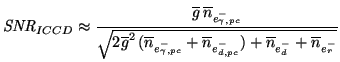$$\mathit{SNR}_{ICCD}\approx \frac{\overline{g}\,\overline{n}_{e^{-... ...overline{n}_{e^{-}_{d,pc}})+\overline{n}_{e^{-}_{d}}+\overline{n}_{e^{-}_{r}}}}$$ (3.38)

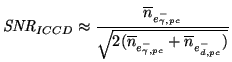
As seen, increasing the gain of the image intensifier makes the CCD noise-sources negligible, but does not increase the $\mathit{SNR}$. For very high gain, Equation 3.38 is reduced to:

$$\mathit{SNR}_{ICCD}\approx \frac{\overline{n}_{e^{-}_{\gamma,pc}}}{\sqrt{ 2(\overline{n}_{e^{-}_{\gamma,pc}}+\overline{n}_{e^{-}_{d,pc}})}}$$ (3.39)

Threshold of detection and maximum signal

The threshold of detection is usually defined as $\mathit{SNR}=2$ while the Noise Equivalent Exposure, $\mathit{NEE}$, is obtained when $\mathit{SNR}=1$. The maximum signal, or Saturation Equivalent Exposure (SEE) is obtained when the charge well capacity, $n_{e^{-}_{max}}$, is reached. This occurs when:

$$n_{e^{-}_{\gamma}} \ge n_{e^{-}_{max}}- n_{e^{-}_{d}}$$ (3.40)

In most cases the maximum charge-well capacity, $\mathit{DN}_{SEE}$, is matched to the maximum ADC output $\mathit{DN}_{max}$. For the ICCD case, apart from the condition above, there is also a saturation level for the image intensifier to be considered. On the other hand, the high-voltage for the intensifier can be gated, acting like an electronic shutter.

Dynamic range

The Dynamic Range, $\mathit{DR}$, is defined as the peak signal divided by the RMS noise and the DC-bias-level, $\mathit{DN}_{DC}$, (if any). The minimum ADC output, $\mathit{DN}_{min}$, is subtracted in the case of a signed integer output. $\mathit{DR}$ is usually expressed in decibels.

$$\mathit{DR}= 20 \log_{10} \left( \frac{\mathit{DN}_{SEE}-\mathit{DN}_{min}} {\mathit{DN}_{DC}+\mathit{DN}_{NEE}-\mathit{DN}_{min}} \right) [dB]$$ (3.41)

An approximate theoretical value for $\mathit{DR}$ is obtained by dividing the maximum signal (Equation 3.40) by the total noise, $\langle n_{e^{-}_{tot}} \rangle$, which is found in Equations 3.26 and 3.37 for the CCD and ICCD case respectively.)

$$\mathit{DR}\approx 20 \log_{10} \frac{n_{e^{-}_{max}}- n_{e^{-}_{d}}}{\langle n_{e^{-}_{tot}} \rangle }\ [dB]$$ (3.42)